02-学习速率
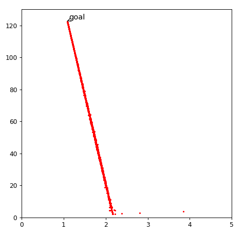
考察学习速率与收敛的关系
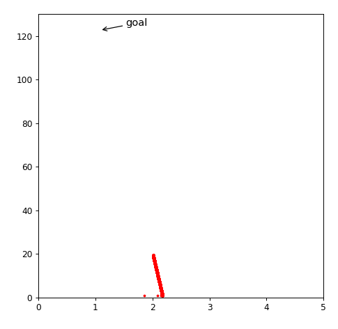
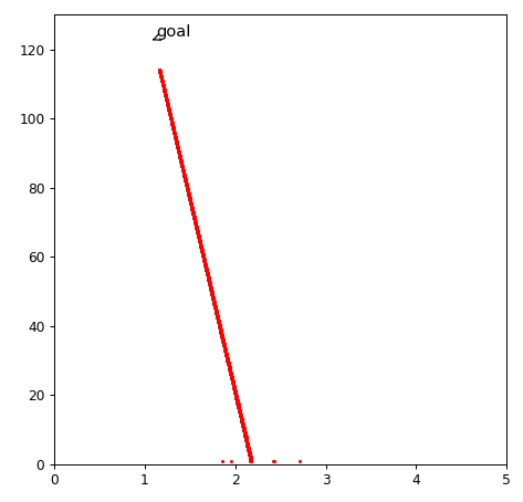
目标点: m = 1.085, b = 122.675
learningrate = 0.000001
10000次迭代
 1
 2
 3
 4
 5
 6
 7
 8
 9
10
11
12
13
14
15
16
17
18
19
20
21
22
23
24
25 | import numpy as np
data = np.array([
[80,200],
[95,230],
[104,245],
[112,247],
[125,259],
[135,262]
])
feature = data[:,0:1]
ones = np.ones((len(feature),1))
Feature = np.hstack((feature ,ones))
Label = data[:,-1:]
weight = np.ones((2,1))
bhistory = []
mhistory = []
learningrate = 0.00001
def gradentdecent():
global weight
weight = weight - learningrate* np.dot(Feature.T,(np.dot(Feature,weight)-Label))
for i in range(1000000):
gradentdecent()
mhistory.append(weight[0][0])
bhistory.append(weight[1][0])
|
 1
 2
 3
 4
 5
 6
 7
 8
 9
10
11
12 | import matplotlib.pyplot as plt
%matplotlib notebook
fig = plt.figure(figsize=(6, 6), dpi=80)
plt.scatter(mhistory,bhistory,c='r',marker='o',s=4.,label='like')
plt.ylim(0,130)
plt.xlim(0,5)
plt.annotate('goal',
xy=(1.085, 122.675), xytext=(+3, +3),
textcoords='offset points', fontsize=12,
arrowprops=dict(arrowstyle="->"))
plt.show()
|
如何找到合适的learningrate,如何优化学习速率?
目前有超级都的learningrate优化的框架和论文,
- adam https://ruder.io/optimizing-gradient-descent/
- adagrad https://medium.com/konvergen/an-introduction-to-adagrad-f130ae871827
- RMSProp https://towardsdatascience.com/understanding-rmsprop-faster-neural-network-learning-62e116fcf29a
- Momentum https://engmrk.com/gradient-descent-with-momentum/
非常多,建议大家如果有兴趣就去读读论文。 算法工程师干的是就是搞个好算法,优化收敛和学习速度。
这些算法的思想原则都非常简单, 我们也可以写一个类似的算法。
学习速率分析
什么是好的学习速率?
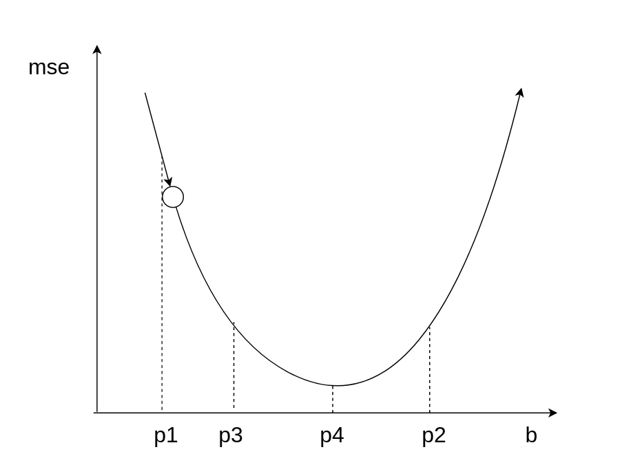
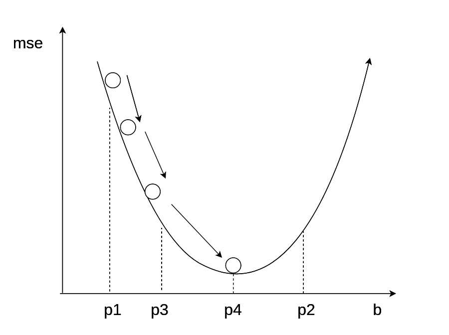
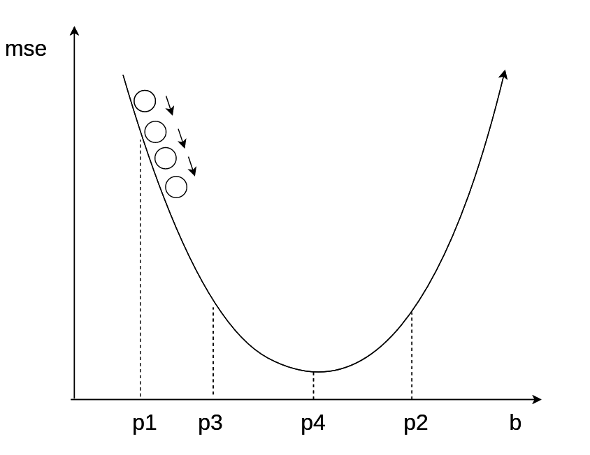
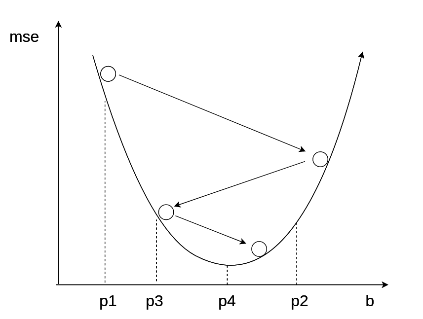
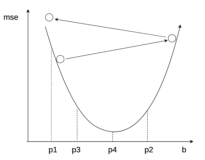
学习率优化算法-HeiMa法
- 每一次梯度下降后,计算当前的mse,并且存储起来
- 对比最近两次的mse,计算他们的差值
- 如果mse变大,说明步子太大,学习速率需要降低,learningrate = learningrate / 2
- 如果mse变小,说明步子没问题,看能不能走的再快一点,learningrate = learningrate × 1.05%
- 重复上述步骤
 1
 2
 3
 4
 5
 6
 7
 8
 9
10
11
12
13
14
15
16
17
18
19
20
21
22
23
24
25
26
27
28
29
30
31
32
33
34 | import numpy as np
data = np.array([
[80,200],
[95,230],
[104,245],
[112,247],
[125,259],
[135,262]
])
feature = data[:,0:1]
ones = np.ones((len(feature),1))
Feature = np.hstack((feature ,ones))
Label = data[:,-1:]
weight = np.ones((2,1))
bhistory = []
mhistory = []
msehistory = []
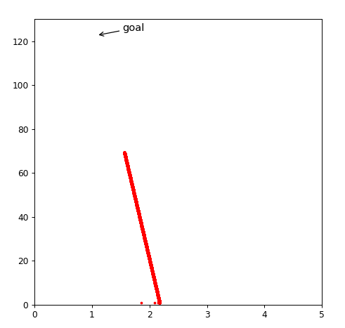
learningrate = 0.00002
def gradentdecent():
global weight,learningrate
mse = np.sum(np.power((np.dot(Feature,weight)-Label),2))
msehistory.append(mse)
if len(msehistory)>=2:
if(msehistory[-1]>msehistory[-2]):
learningrate = learningrate /2
else :
learningrate = learningrate * 1.1
weight = weight - learningrate* np.dot(Feature.T,(np.dot(Feature,weight)-Label))
for i in range(500000):
gradentdecent()
mhistory.append(weight[0][0])
bhistory.append(weight[1][0])
|
 1
 2
 3
 4
 5
 6
 7
 8
 9
10
11
12 | import matplotlib.pyplot as plt
%matplotlib notebook
fig = plt.figure(figsize=(6, 6), dpi=80)
plt.scatter(mhistory,bhistory,c='r',marker='o',s=2.,label='like')
plt.ylim(0,130)
plt.xlim(0,5)
plt.annotate('goal',
xy=(1.085, 122.675), xytext=(+3, +3),
textcoords='offset points', fontsize=12,
arrowprops=dict(arrowstyle="->"))
plt.show()
|
50万次,就很接近了目标点了。
Heima算法升级版本
 1
 2
 3
 4
 5
 6
 7
 8
 9
10
11
12
13
14
15
16
17
18
19
20
21
22
23
24
25
26
27
28
29
30
31
32
33
34
35
36
37
38
39
40
41
42
43
44
45
46
47 | import numpy as np
data = np.array([
[80,200],
[95,230],
[104,245],
[112,247],
[125,259],
[135,262]
])
feature = data[:,0:1]
ones = np.ones((len(feature),1))
Feature = np.hstack((feature ,ones))
Label = data[:,-1:]
weight = np.ones((2,1))
bhistory = []
mhistory = []
msehistory = []
learningrate = 10
l_b=0.0
l_m = 0
##关键代码
changeweight = np.zeros((2,1))
def gradentdecent():
global changeweight
global weight,learningrate
mse = np.sum(np.power((np.dot(Feature,weight)-Label),2))
msehistory.append(mse)
if len(msehistory)>=2:
if(msehistory[-1]>msehistory[-2]):
learningrate = learningrate /2
else :
learningrate = learningrate * 1.1
change = np.dot(Feature.T,(np.dot(Feature,weight)-Label))
###关键代码
changeweight = changeweight + change**2
weight = weight - learningrate* change/np.sqrt(changeweight)
###关键代码
for i in range(10000):
gradentdecent()
mhistory.append(weight[0][0])
bhistory.append(weight[1][0])
|
 1
 2
 3
 4
 5
 6
 7
 8
 9
10
11
12 | import matplotlib.pyplot as plt
%matplotlib notebook
fig = plt.figure(figsize=(6, 6), dpi=80)
plt.scatter(mhistory,bhistory,c='r',marker='o',s=2.,label='like')
plt.ylim(0,130)
plt.xlim(0,5)
plt.annotate('goal',
xy=(1.085, 122.675), xytext=(+3, +3),
textcoords='offset points', fontsize=12,
arrowprops=dict(arrowstyle="->"))
plt.show()
|
一万次迭代,到达目标
考虑历史因素,类似pid算法的思想。对于之前更新很多的,历史变化大,相对就可以慢一点,而对那些没怎么更新过的,就可以给一个大一些的学习率。