02-交叉熵

预测分布越接近真实的分布，交叉熵越小，当预测分布等于真实分布时，交叉熵最小，此时交叉熵的值等同于熵。所以，交叉熵提供了一种衡量两个分布之间差异大小的方式，常用来作为神经网络的损失函数。当预测分布跟真实分布（人工标注结果）相差很大时，交叉熵就大；当随着训练的进行预测分布越来越接近真实分布时，交叉熵就逐渐减小。

$$CrossEntropy = - ((Actual) * log(Guess) + (1-Actual )*log（1-Guess))$$

$$Entropy = -\dfrac {m}{m+n}\log (\dfrac {m}{m+n})-\dfrac {n}{m+n}\log (\dfrac {n}{m+n})$$

$$Entropy = -(Actual)*log(Actual) - (1-Actual)*log(1-Actual)$$

from sympy import *  #导入计算库
x, y, z = symbols('x, y, z') #声明变量x,y,z
init_printing(pretty_print=True) #初始化latex显示
limit(log(x), x, 1)      0*log(0) = 0

小明： 深圳明天晴天的概率是 80%

小刚： 深圳明天晴天的概率是 50%

天气预报预测的 明天晴天的概率是65%， 小明和小刚谁预测的准确度高

谁的交叉熵小，谁的预测准确性高

$-0.65* log(0.8) - 0.35*log(0.2) = 0.708346577706171$

$-0.65* log(0.5)-0.35* log(0.5) = 0.693147180559945$

天气预报预测的 明天晴天的概率是1， 小明和小刚谁预测的准确度高

$-1* log(0.8) -0*log(0.2) =0.22314355131421$

$-1* log(0.5) -0*log(0.5) = 0.693147180559945$

交叉熵梯度下降

现在逻辑回归的问题就变成了一个数学问题，

如何降低交叉熵的值。

$$Guess = \dfrac {1}{1+e^{-\left( m*x + b\right) }}$$

$$CrossEntropy = - ((Actual) * log(Guess) + (1-Actual )*log（1-Guess))$$

上面是一个点的数据，我们现在需要多个点的交叉熵

$$CrossEntropy = - \sum ^{n}_{n=1} ((Actual_i) * log(Guess_i) + (1-Actual_i )*log（1-Guess_i))$$

$$error = -\sum ^{n}_{n=1} ((Actual_i) * log(\dfrac {1}{1+e^{-\left( m*x_i + b\right) }}) + (1-Actual_i )*log（1-\dfrac {1}{1+e^{-\left( m*x_i + b\right) }}))$$

分别对m和b求偏导数，让m和b的偏导数值接近于0。

expr = - Sum( Actual_i* log(1/(1+exp(-(m*x_i+b)))) + (1-Actual_i)* log(1 - 1/(1+exp(-(m*x_i+b)))) , (x_i, 1, n))

$\displaystyle - \sum_{x_{i}=1}^{n} \left(Actual_{i} \log{\left(\frac{1}{e^{- b - m x_{i}} + 1} \right)} + \left(1 - Actual_{i}\right) \log{\left(1 - \frac{1}{e^{- b - m x_{i}} + 1} \right)}\right)$

diff(expr,m)

$\displaystyle - \sum_{x_{i}=1}^{n} \left(\frac{Actual_{i} x_{i} e^{- b - m x_{i}}}{e^{- b - m x_{i}} + 1} - \frac{x_{i} \left(1 - Actual_{i}\right) e^{- b - m x_{i}}}{\left(1 - \frac{1}{e^{- b - m x_{i}} + 1}\right) \left(e^{- b - m x_{i}} + 1\right)^{2}}\right)$

diff(expr,b)

$\displaystyle - \sum_{x_{i}=1}^{n} \left(\frac{Actual_{i} e^{- b - m x_{i}}}{e^{- b - m x_{i}} + 1} - \frac{\left(1 - Actual_{i}\right) e^{- b - m x_{i}}}{\left(1 - \frac{1}{e^{- b - m x_{i}} + 1}\right) \left(e^{- b - m x_{i}} + 1\right)^{2}}\right)$

simplify(diff(expr,b))

$\displaystyle \sum_{x_{i}=1}^{n} \left(- \frac{Actual_{i}}{e^{b + m x_{i}} + 1} - \frac{Actual_{i}}{e^{- b - m x_{i}} + 1} + \frac{1}{e^{- b - m x_{i}} + 1}\right)$

(simplify(diff(expr,m)))

$\displaystyle \sum_{x_{i}=1}^{n} x_{i} \left(- \frac{Actual_{i}}{e^{b + m x_{i}} + 1} - \frac{Actual_{i}}{e^{- b - m x_{i}} + 1} + \frac{1}{e^{- b - m x_{i}} + 1}\right)$

$\dfrac {CrossEntropy}{\Delta b} = Guess_i - Actual_i$

$\dfrac {CrossEntropy}{\Delta m} = x_i*(Guess_i-Actual_i)$

交叉熵梯度下降矩阵表达

线性回归误差对m和b的偏导数$∂_1$ 、逻辑回归误差对m和b的偏导数$∂_2$ 有以下公式：

$$∂_1 = Feature.T * (Feature * Weight - Label)$$

$$∂_2 = Feature.T * (sigmoid(Feature * Weight) - Label)$$

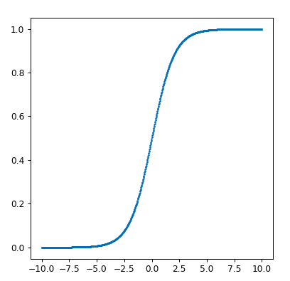
sigmoid 函数

%matplotlib notebook 
import matplotlib.pyplot as plt #导包
import numpy as np
fig = plt.figure(figsize=(5, 5), dpi=80)
X = np.linspace(-10,10,1000)
y = 1/(1+np.exp(-X))
plt.scatter(X,y,s=1)
plt.show()

代码实现

def sigmoid(z):
    return 1 / (1 + np.exp(-z))

import numpy as np
data = np.array([
    [5,0],
    [15,0],
    [25,1],
    [35,1],
    [45,1],
     [55,1]
])
feature = data[:,0:1]
ones = np.ones((len(feature),1))
Feature = np.hstack((feature ,ones))
Label = data[:,-1:]
weight = np.ones((2,1))

bhistory = []
mhistory = []
msehistory = []
learningrate = 0.0001
l_b=0.0
l_m = 0

##关键代码
changeweight  = np.zeros((2,1))

def sigmoid(z):
    return 1 / (1 + np.exp(-z))

def gradentdecent():
    global changeweight
    global weight,learningrate
    mse = np.sum(np.power((sigmoid(np.dot(Feature,weight))-Label),2))
    msehistory.append(mse)
    if len(msehistory)>=2:
        if(msehistory[-1]>msehistory[-2]):
            learningrate = learningrate /2
        else :
            learningrate = learningrate * 1.1

    change = np.dot(Feature.T,(sigmoid(np.dot(Feature,weight))-Label))
    ###关键代码
    changeweight = changeweight + change**2       
    weight = weight - learningrate* change/np.sqrt(changeweight)
    ###关键代码


for i in range(10000):
    gradentdecent()
    mhistory.append(weight[0][0])
    bhistory.append(weight[1][0])

np.set_printoptions(suppress=True)
print(sigmoid(np.dot(Feature,weight)))

预测

predict = np.array([[10,1]])
print(sigmoid(np.dot(predict,weight)))